How can we solve High-Speed Printing Defect Detection?
Product packaging covers are printed with branding and marketing information (refer to Figure 1). A specialised large-scale printing system prints on the packaging material rolls at high speed, which run several meters in length. Any improper setup, a minor misalignment, or the printing process noise itself can introduce defects while printing. These defects have no defined shape or form and can be anything from lines to small color splashes to CMY colour channel misalignments, etc. A defect can be defined as any difference between the intended printing and the actual printing, excluding the process noise (process noise is a slight deviation introduced in printing as the sheet stretches and flaps because of high-speed sheet rollers). Refer to Figure 2 for some examples of printing defects.

These defects can greatly affect the product brand value if it goes undetected and lands at the end consumer’s hand. Hence, early detection of defects is crucial. As the printing happens at high speed, manual inspection gets challenging in spotting defects. Thus the need of an auto-inspection system becomes very important for such use cases.
Problem Statement
The printing speed is somewhere between 2-5 meters per second, which results in a frame rate of 10-20 frames per second. This rate is very high for a human to spot small defects which spread over a few pixels, that too from an image frame of 3000 x 5000 pixels resolution. Hence auto detection is the only way which can bring value to quality assurance. Thus the above requirements can be mapped into following problem statement:
“Using the reference frame (or image), detect any deviations present in the test frame (or image), excluding minor deviations introduced by printing process noise. Processing time should be atleast 100 miliseconds per test frame”

Challenges
- Small Defect Footprint: The defect footprint is tiny compared to the image frame. For example, the defect line width can be as small as 2 pixels whereas image frame is of high resolution i.e. 3000 x 5000 pixels.
- Processing time vs High Resolution Input Frame: The processing time requirement is sub-100 milliseconds to process a frame of 3000 x 5000 resolution. Down-scaling the frame resolution in order to reduce the processing time can make smaller defects to go unnoticed.
- Process Noise: Although process noise is acceptable, it introduces visual variations w.r.t reference frame which makes pixel-to-pixel comparison futile (even with image registration techniques, see Image Registration Approach).
Approach
During the project course following approaches were tried out. We began with Image Registration techniques, followed by deep learning models. The below sections describe this journey and our observations.
Deep Learning using CNN
CNNs have proven to identify patterns in images by auto learning the necessary feature extraction filters (spread over several hidden layers). Also the CNN computations are optimized for GPUs, a low processing time can be expected. Convolution operations are performed on small image patches, whose size is defined by the convolution kernel width. Since these operations are independent, huge speedup is obtained using GPUs. We used Tensorflow, a deep learning framework which makes use of optimized GPU operations under the hood.
Since GPU RAM determines the input size (and output size) that can be processed in one forward pass (the flow of an image through the different layers of a CNN), it was required that we split the high resolution test frame (and hence the reference frame) into small tiles of 256×256 resolution each.
Siamese Network
- Siamese CNN models are a preferred choice when it comes to image comparison. In our case, we need to compare the test frame with the reference frame and identify any defects. Therefore, the Siamese network was our first choice when it comes to CNN.
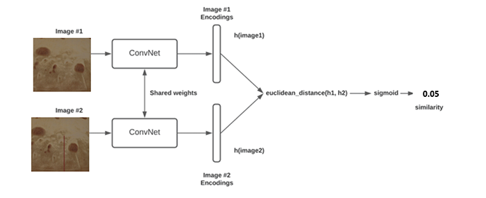
Image-Siamese Network for defect identification
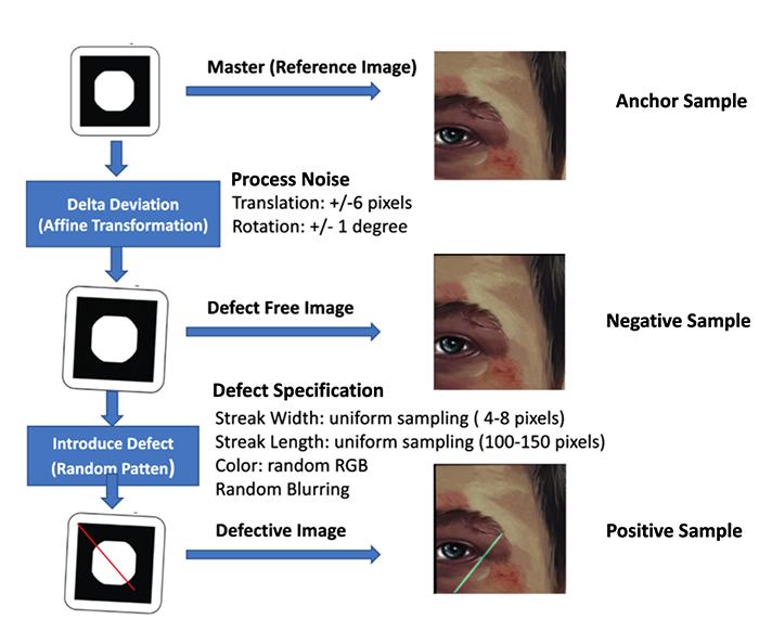
- We trained a Siamese network following a Tensorflow-Keras tutorial here. To train a siamese network, a dataset must be prepared in triplet form consisting of an Anchor, a Positive example, and a Negative example.
- Where Anchor is the reference image.
- Positive sample is a test sample which contains the print defect and process noise.
- Negative sample is a test sample which has no defect, but just the process noise.
- The dataset creation process is shown below:
- Random images from the internet were collected.
- For the Anchor sample, crops or tiles of shape 256×256 were randomly sampled from the collected images.
- For the negative sample, artificial noise was introduced to the anchor sample. Random rotation (-/+ 1 degree) and random translation (-/+ 6 pixels) were added to the anchor images to obtain the negative sample.
- For the positive sample, random colored lines and splashes were added to represent defect lines in the negative sample.
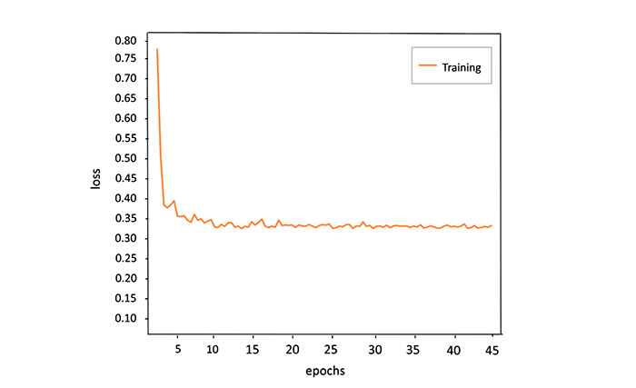
- It was observed during the training process that the model could not converge beyond a specific loss. This observation holds true even for different CNN backbones and varying hyperparameters.
-
- We hypothesize two reasons that might be playing against model learning:
- Small Defect Signature: Although the Siamese network has been proven effective in obtaining similarity between two images, in our case, the Anchor and Positive images are already visually very similar, apart from a minor defect signature.
- Process Noise Overshadowing Defect: As the test images undergo non-rigid deformation due to process noise, and as we instruct the model to accept the process noise through Anchor and Negative samples, the visual variations of process noise must be overshadowing the visual variations of defects.
- We further hypothesize that because of the above two reasons, the image encoding/features outputted by the Siamese network fails to capture the defect signature effectively, especially for small lines and colour splashes which are a few pixels wide.
Binary Classifier With 6-Channel Input Image
- As the Siamese network failed to learn the defect encodings effectively, we felt a need to extract effective features at the very beginning of the network from the overlap of reference and test image (just like a person would do to spot the difference)
- Overlapping can be achieved by concatenating the test and reference images along the channel axis, forming a 6-channel image that will be an input to the CNN.
- A binary classifier CNN (with sigmoid as the last activation layer) will produce “True” for the input Anchor-Positive pair and “False” for the input Anchor-Negative pair. A pair is now a 6-channel image obtained as stated above.
- We used EfficientNetB0 from Tensorflow as the base network and used the following parameters while instantiating the model:
- input_shape = (None, 256, 256, 6)
- classes = 1
- classifier_activation = “sigmoid”
- This new scheme helped achieve model convergence and 98% accuracy on the validation dataset.
- We hypothesize two reasons that might be playing against model learning:
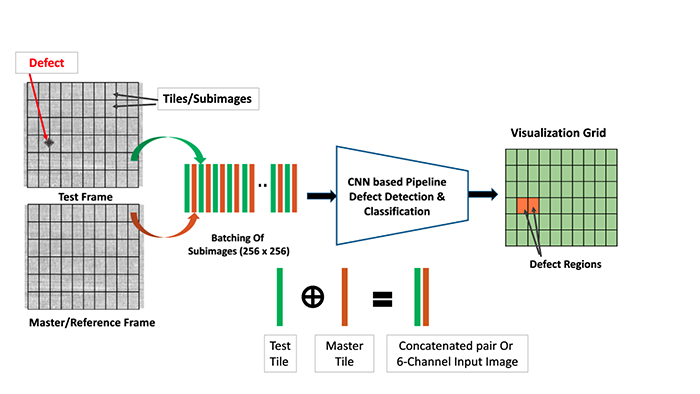
New scheme to compare tiles for defect detection, where filters in early layers learn to ignore differences due to process noise and focuses on actual defects
-
-
Optimization for Speed
The printing defect detection required a processing rate of 10-20 frames a second, where each frame is a “high resolution” image of 3000×5000 pixels resolution at minimum. Here “high resolution” signifies that input image dimension is high w.r.t conventional CNN applications where input image resolution is usually below 1024 x 1024 pixels. To obtain the desired processing rate of at least 10-20 fps, the following optimization options were possible:
GPU-based Post-Processing Operations
The post-processing operation involved the following operations:
- Tile Formation and Extraction: tile formation and extraction must be performed for reference and test frames, where each tile is 256×256 crop.
- Tile Concatenation: Tile from reference and test frames will be concatenated based on their respective positions along the channel axis.
- Batch Formation of Concatenated Tiles: Batch processing of 6-Channel image (obtained by respective tile concatenation) is faster than processing of single 6-Channel image.
Above operations were initially implemented in OpenCV and were executed on CPU, a GPU equivalent will significantly speed up the operation. This transfer of execution to GPU can be achieved by either writing a customized CUDA kernel OR using Tensorflow Graph as explained below.
Use Of TensorFlow Graph Execution Instead Of Eager Execution
Tensorflow by default makes use of eager flow, where Python Interpreter orchestrates the execution and hence some latency is introduced along the way. Graph execution is a way by which a computation graph is created describing the user’s operation, which can be executed faster without involving python interpreter. More details can be found in the introduction on TF Graph blog. Below is the implementation of tensorflow:
Summary
Using the optimization techniques mentioned above and GPUs such as GTX1660ti and RTX A4000, we achieved a performance of less than one second (approximately 0.9 seconds) per frame. This is a significant improvement from the starting point of over 20 seconds of execution time per frame. For further improvement below are planned methods for speed optimizations.
Other Planned Methods for Speed Optimization
Our objective is to take execution speed down to 100 milliseconds per frame, and towards that goal below are techniques we want to make use of:
- Use of CUDA Pinned Memory Transfer: for test images, Pinned memory will be used to transfer subsequent test frames to GPU. Pinned memory is a type of memory that remains in a fixed location in the system’s physical memory and is not subject to virtual memory paging. This arrangement has several advantages over regular pageable memory, like faster transfer of memory, improved concurrency, and reduced CPU overhead.
- Use TensorFlowRT: TensorFlow RT is optimized for fast inference performance and is designed to take full advantage of the hardware acceleration available on GPU. The optimization primarily involves lowering the precision from default FP32 to FP16 or even INT8, which results in faster computation and a lower model footprint.
- Use Of Multi-GPU configuration: Although having a multi-GPU system is costlier, it improves speed. The high-resolution master and test frames can be split into parts, and the corresponding defect detection can be spread over multiple GPUs to further speed up time.
-





https://t.me/s/Online_1_xbet/285
https://t.me/s/Online_1_xbet/3075
https://t.me/s/Official_1xbet_1xbet
https://t.me/rating_online/6
https://t.me/rating_online/1
https://t.me/s/rating_online/5
https://t.me/s/rating_online/3
https://t.me/s/rating_online/9
https://t.me/rating_online/8
https://t.me/rating_online/7
https://t.me/s/rating_online/1
https://t.me/rating_online
https://t.me/Online_1_xbet/2857
https://t.me/Online_1_xbet/3355
https://t.me/Online_1_xbet/2637
https://t.me/Online_1_xbet/2354
https://t.me/Online_1_xbet/3426
https://t.me/Online_1_xbet/2825
https://t.me/Online_1_xbet/2573
https://t.me/Online_1_xbet/1961
https://t.me/Online_1_xbet/2517
https://t.me/Online_1_xbet/2319
https://t.me/Official_1xbet_1xbet/s/1365
https://t.me/Official_1xbet_1xbet/s/1094
https://t.me/Official_1xbet_1xbet/s/914
https://t.me/Official_1xbet_1xbet/s/559
https://t.me/Official_1xbet_1xbet/s/983
https://t.me/Official_1xbet_1xbet/s/1010
https://t.me/Official_1xbet_1xbet/s/1009
https://t.me/Official_1xbet_1xbet/s/867
https://t.me/Official_1xbet_1xbet/s/1426
https://t.me/Official_1xbet_1xbet/s/1324
https://t.me/Official_1xbet_1xbet/s/1013
https://t.me/Official_1xbet_1xbet/s/442
https://t.me/Official_1xbet_1xbet/s/1509
https://t.me/Official_1xbet_1xbet/s/1238
https://t.me/Official_1xbet_1xbet/s/920
https://t.me/Official_1xbet_1xbet/s/1120
https://t.me/Official_1xbet_1xbet/s/1510
https://t.me/Official_1xbet_1xbet/s/1112
https://t.me/Official_1xbet_1xbet/s/411
https://t.me/Official_1xbet_1xbet/s/815
https://t.me/Official_1xbet_1xbet/s/655
https://t.me/Official_1xbet_1xbet/s/440
https://t.me/Official_1xbet_1xbet/s/989
https://t.me/Official_1xbet_1xbet/s/172
https://t.me/Official_1xbet_1xbet/s/1312
https://t.me/Official_1xbet_1xbet/s/446
https://t.me/Official_1xbet_1xbet/s/1329
https://t.me/Official_1xbet_1xbet/s/1211
https://t.me/Official_1xbet_1xbet/s/152
https://t.me/Official_1xbet_1xbet/s/790
https://t.me/Official_1xbet_1xbet/s/194
https://t.me/Official_1xbet_1xbet/s/1034
https://t.me/Official_1xbet_1xbet/s/378
https://t.me/Official_1xbet_1xbet/s/197
https://t.me/Official_1xbet_1xbet/s/516
https://t.me/Official_1xbet_1xbet/s/302
https://t.me/Official_1xbet_1xbet/s/971
https://t.me/Official_1xbet_1xbet/s/561
https://t.me/Official_1xbet_1xbet/s/269
https://t.me/Official_1xbet_1xbet/s/455
https://t.me/Official_1xbet_1xbet/s/474
https://t.me/Official_1xbet_1xbet/s/304
https://t.me/Official_1xbet_1xbet/s/522
https://t.me/Official_1xbet_1xbet/s/168
https://t.me/Official_1xbet_1xbet/s/544
https://t.me/Official_1xbet_1xbet/s/591
https://t.me/Official_1xbet_1xbet/s/956
https://t.me/Official_1xbet_1xbet/1608
https://t.me/s/Official_1xbet_1xbet/1596
https://t.me/s/Official_1xbet_1xbet/1705
https://t.me/Official_1xbet_1xbet/1829
https://t.me/s/Official_1xbet_1xbet/1720
https://t.me/s/Official_1xbet_1xbet/1762
https://t.me/Official_1xbet_1xbet/1799
https://t.me/s/Official_1xbet_1xbet/1706
https://t.me/Official_1xbet_1xbet/1847
https://t.me/s/Official_1xbet_1xbet/1722
https://t.me/s/Official_1xbet_1xbet/1597
https://t.me/s/Official_1xbet_1xbet/1605
https://t.me/s/Official_1xbet_1xbet/1844
https://t.me/s/Official_1xbet_1xbet/1759
https://t.me/Official_1xbet_1xbet/1671
https://t.me/s/Official_1xbet_1xbet/1785
https://t.me/Official_1xbet_1xbet/1691
https://t.me/Official_1xbet_1xbet/1794
https://t.me/Official_1xbet_1xbet/1661
https://t.me/Official_1xbet_1xbet/1618
https://t.me/s/Official_1xbet_1xbet/1648
https://t.me/Official_1xbet_1xbet/1809
https://t.me/s/Official_1xbet_1xbet/1631
https://t.me/s/Official_1xbet_1xbet/1834
https://t.me/s/Official_1xbet_1xbet/1650
https://t.me/s/Official_1xbet_1xbet/1818
https://t.me/Official_1xbet_1xbet/1791
https://t.me/s/Official_1xbet_1xbet/1830
https://t.me/s/Official_1xbet_1xbet/1637
https://t.me/Official_1xbet_1xbet/1858
https://t.me/s/Official_1xbet_1xbet/1838
https://t.me/Official_1xbet_1xbet/1807
https://t.me/Official_1xbet_1xbet/1605
https://t.me/Official_1xbet_1xbet/1850
https://t.me/s/Official_1xbet_1xbet/1763
https://t.me/Official_1xbet_1xbet/1659
https://t.me/s/Official_1xbet_1xbet/1753
https://t.me/Official_1xbet_1xbet/1642
https://t.me/Official_1xbet_1xbet/1848
https://t.me/s/Official_1xbet_1xbet/1848
https://t.me/s/Official_1xbet_1xbet/1836
https://t.me/Official_1xbet_1xbet/1702
https://t.me/Official_1xbet_1xbet/1752
https://t.me/Official_1xbet_1xbet/1833
https://t.me/s/Official_1xbet_1xbet/1723
https://t.me/Official_1xbet_1xbet/1801
https://t.me/Official_1xbet_1xbet/1812
https://t.me/s/Official_1xbet_1xbet/1642
https://t.me/s/Official_1xbet_1xbet/1682
https://t.me/Official_1xbet_1xbet/1784
https://t.me/s/Official_1xbet_1xbet/1636
https://t.me/s/Official_1xbet_1xbet/1792
https://t.me/Official_1xbet_1xbet/1745
https://t.me/s/Official_1xbet_1xbet/1761
https://t.me/s/Official_1xbet_1xbet/1686
https://t.me/Official_1xbet_1xbet/1697
https://t.me/s/Official_1xbet_1xbet/1795
https://t.me/s/Official_1xbet_1xbet/1679
https://t.me/Official_1xbet_1xbet/1797
https://t.me/Official_1xbet_1xbet/1606
https://t.me/s/Official_1xbet_1xbet/1858
https://t.me/Official_1xbet_1xbet/1798
https://t.me/s/Official_1xbet_1xbet/1688
https://t.me/s/Official_1xbet_1xbet/1778
https://t.me/Official_1xbet_1xbet/1620
https://t.me/Official_1xbet_1xbet/1843
https://t.me/s/Official_1xbet_1xbet/1816
https://t.me/s/topslotov
https://t.me/s/official_1win_aviator
https://t.me/s/reiting_top10_casino/5
https://t.me/reiting_top10_casino/3
https://t.me/s/reiting_top10_casino/4
https://t.me/s/reiting_top10_casino
https://t.me/reiting_top10_casino/2
https://t.me/reiting_top10_casino/9
https://t.me/reiting_top10_casino/4
https://t.me/reiting_top10_casino/10
https://t.me/s/reiting_top10_casino/10
https://t.me/s/reiting_top10_casino/3
https://t.me/reiting_top10_casino/6
https://t.me/reiting_top10_casino/7
https://t.me/reiting_top10_casino/8
https://t.me/reiting_top10_casino
https://t.me/s/reiting_top10_casino/6
https://t.me/s/reiting_top10_casino/7
https://t.me/s/reiting_top10_casino/8
https://t.me/s/reiting_top10_casino/9
https://t.me/s/reiting_top10_casino/2
https://t.me/reiting_top10_casino/5
https://t.me/s/Gaming_1xbet
https://t.me/s/PlayCasino_1xbet
https://t.me/s/PlayCasino_1win
https://t.me/s/PlayCasino_1xbet
https://t.me/s/PlayCasino_1win
https://t.me/s/ofitsialniy_1win/33/kes
https://t.me/s/iw_1xbet
https://t.me/s/Official_beefcasino
https://t.me/s/ofitsialniy_1win
https://t.me/bs_1xbet/50
https://t.me/s/bs_1xbet/40
https://t.me/s/bs_1xbet/38
https://t.me/s/bs_1xbet/30
https://t.me/s/bs_1xbet/32
https://t.me/s/bs_1xbet/6
https://t.me/s/bs_1xbet/43
https://t.me/s/bs_1xbet/23
https://t.me/s/bs_1xbet/36
https://t.me/s/bs_1xbet/7
https://t.me/bs_1xbet/49
https://t.me/bs_1xbet/3
https://t.me/s/bs_1xbet/29
https://t.me/bs_1xbet/35
https://t.me/bs_1xbet/41
https://t.me/s/bs_1xbet/20
https://t.me/bs_1xbet/10
https://t.me/s/bs_1xbet/15
https://t.me/s/bs_1xbet/5
https://t.me/bs_1xbet/41
https://t.me/s/bs_1xbet/20
https://t.me/bs_1xbet/8
https://t.me/s/bs_1xbet/19
https://t.me/bs_1xbet/20
https://t.me/bs_1xbet/20
https://t.me/s/bs_1xbet/42
https://t.me/s/bs_1xbet/38
https://t.me/bs_1xbet/33
https://t.me/bs_1xbet/30
https://t.me/bs_1xbet/9
https://t.me/s/bs_1xbet/38
https://t.me/bs_1xbet/32
https://t.me/bs_1xbet/38
https://t.me/s/bs_1xbet/31
https://t.me/bs_1xbet/33
https://t.me/bs_1xbet/7
https://t.me/s/bs_1xbet/51
https://t.me/bs_1xbet/29
https://t.me/s/bs_1xbet/47
https://t.me/bs_1xbet/27
https://t.me/s/bs_1xbet/5
https://t.me/s/bs_1xbet/22
https://t.me/s/jw_1xbet/610
https://t.me/s/jw_1xbet/45
https://t.me/jw_1xbet/842
https://t.me/jw_1xbet/212
https://t.me/jw_1xbet/530
https://t.me/s/jw_1xbet/728
https://t.me/s/bs_1Win/561
https://t.me/s/bs_1Win/803
https://t.me/bs_1Win/806
https://t.me/s/bs_1Win/416
https://t.me/s/bs_1Win/398
https://t.me/bs_1Win/538
https://t.me/s/bs_1Win/1081
https://t.me/bs_1Win/370
https://t.me/bs_1Win/1175
https://t.me/s/bs_1Win/622
https://t.me/bs_1Win/1133
https://t.me/bs_1Win/502
https://t.me/s/Official_mellstroy_casino/10
https://t.me/s/Official_mellstroy_casino/29
https://t.me/Official_mellstroy_casino/10
https://t.me/s/Beefcasino_rus/30
https://t.me/s/Official_mellstroy_casino/56
https://t.me/Official_mellstroy_casino/43
https://t.me/s/Official_mellstroy_casino/48
https://t.me/Official_mellstroy_casino/18
https://t.me/s/Official_mellstroy_casino/23
https://t.me/s/Official_mellstroy_casino/53
https://t.me/s/Official_mellstroy_casino/35
https://t.me/Official_mellstroy_casino/15
https://t.me/Official_mellstroy_casino/29
https://t.me/Official_mellstroy_casino/56
https://t.me/s/Best_promocode_rus/594
https://t.me/s/Best_promocode_rus/2368
https://t.me/Beefcasino_rus/57
https://t.me/s/ud_Kent/55
https://t.me/ud_Pokerdom/64
https://t.me/s/ud_Riobet/54
https://t.me/ud_CatCasino/61
https://t.me/s/ud_Legzo/58
https://t.me/ud_CatCasino/48
https://t.me/s/ud_JoyCasino/54
https://t.me/s/ud_Pin_Up/57
https://t.me/ud_Flagman/47
https://t.me/s/ud_Drip/55
https://t.me/?ud_1Go/60
https://t.me/ud_1xbet/45
https://t.me/s/ud_GGBet/60
https://t.me/s/ud_1xbet/51
https://t.me/ud_Booi/63
https://t.me/ud_DragonMoney/54
https://t.me/s/ud_Pinco/50
https://t.me/s/Beefcasino_rus/59
https://t.me/s/ud_Sol/59
https://t.me/s/ud_Vodka/59
https://t.me/ud_Stake/58
https://t.me/ud_Izzi/63
https://t.me/s/ud_Pinco/56
https://t.me/s/ud_Lex/53
https://t.me/s/ud_Kometa/54
https://t.me/ud_Rox/54
https://t.me/s/ud_Kent/49
https://t.me/s/ud_Fresh/21
https://t.me/s/ud_CatCasino/33
https://t.me/s/ud_MarTin
https://t.me/s/uD_stArda
https://t.me/s/UD_drIp
https://t.me/s/UD_pinCo
https://t.me/s/Ud_GiZbo
https://t.me/s/uD_leoN
https://t.me/s/uD_CASinO_X
https://t.me/s/official_1win_aviator/38
https://t.me/s/Ud_catcasINo
https://t.me/s/UD_VULKAN
https://t.me/official_1win_aviator/89
https://t.me/s/UD_jEt
https://t.me/s/uD_soL
https://t.me/s/Ud_monRo
https://t.me/s/UD_lex
https://t.me/s/tf_1win
https://t.me/s/kta_1win
https://t.me/s/tf_1win
https://t.me/s/kfo_1win
https://t.me/s/UD_vULKAn
https://t.me/s/official_1win_aviator/123
https://t.me/s/Ud_gAMa
https://t.me/s/uD_fLAgmAn
https://t.me/s/UD_pIn_uP
https://t.me/s/UD_gGbET
https://t.me/s/UD_PInco
https://t.me/s/ud_DRagoNmonEY
https://t.me/s/Ud_StarDa
https://t.me/s/ud_MRbIt
https://t.me/s/ud_riObet
https://t.me/s/ud_1xSlOtS
https://t.me/s/ud_keNT
https://t.me/s/uD_mArTIN
https://t.me/s/ke_Starda
https://t.me/s/ke_Stake
https://t.me/s/ke_1Win
https://t.me/official_1win_aviator/76
https://t.me/s/ke_Volna
https://t.me/s/ke_Vulkan
https://t.me/s/ke_Gama
https://t.me/s/ke_CatCasino
https://t.me/s/ke_1Go
https://t.me/s/ke_Booi
https://t.me/s/ke_Izzi
https://t.me/s/ke_Pin_Up
https://t.me/s/ke_mellstroy
https://t.me/s/ke_Pinco
https://t.me/s/ke_PlayFortuna
https://t.me/s/ke_MostBet
https://t.me/s/ke_JoyCasino
https://t.me/s/ke_1xbet
https://t.me/s/kef_Rox
https://t.me/s/ke_Sol
https://t.me/s/ke_Martin
https://t.me/s/ke_MrBit
https://t.me/s/ke_GGBet
https://t.me/s/ke_Irwin
https://t.me/s/ke_Fresh
https://t.me/s/kef_Lex
https://t.me/s/ke_1xSlots
https://t.me/s/kef_beef
https://t.me/s/ke_DragonMoney
https://t.me/s/official_1win_aviator/29
https://t.me/s/ke_Leon
https://t.me/official_1win_aviator/193
https://t.me/s/ke_Casino_X
https://t.me/s/ke_Monro
https://t.me/s/ke_Legzo
https://t.me/s/ke_Pokerdom
https://t.me/s/ke_Riobet
https://t.me/s/ke_Kometa
https://t.me/s/top_kazino_z
https://t.me/s/topcasino_v_rossii
https://t.me/s/a_Top_onlinecasino/2
https://t.me/s/a_Top_onlinecasino/5
https://t.me/s/a_Top_onlinecasino/4
https://t.me/s/a_Top_onlinecasino/15
https://t.me/a_Top_onlinecasino/7
https://t.me/a_Top_onlinecasino/16
https://t.me/a_Top_onlinecasino/5
https://t.me/a_Top_onlinecasino/4
https://t.me/s/a_Top_onlinecasino/3
https://t.me/a_Top_onlinecasino/11
https://t.me/topcasino_rus/
https://t.me/s/official_Irwin_es
https://t.me/s/official_R7_es
https://t.me/s/official_Kent_es
https://t.me/s/official_Drip_ed
https://t.me/s/official_1xSlots_es
https://t.me/s/official_Flagman_es
https://t.me/s/official_Starda_ed
https://t.me/s/official_Lex_ed
https://t.me/s/official_1Go_ed
https://t.me/s/official_Monro_ed
https://t.me/s/official_Sol_es
https://t.me/s/official_Vodka_ed
https://t.me/s/official_MrBit_es
https://t.me/s/official_Drip_es
https://t.me/s/official_JoyCasino_ed
https://t.me/s/official_Legzo_ed
https://t.me/s/official_PlayFortuna_es
https://t.me/s/official_Lex_es
https://t.me/s/official_Daddy_ed
https://t.me/s/official_Riobet_ed
https://t.me/s/official_Gizbo_ed
https://t.me/s/official_Gama_ed
https://t.me/s/official_Pinco_es
https://t.me/s/official_Pokerdom_ed
https://t.me/s/PinUp_egs/16
https://t.me/s/JoyCasino_egs/21
https://t.me/iGaming_live/4668
https://t.me/Legzo_egs/19
https://t.me/Volna_egs/18
https://t.me/Booi_egs/14
https://t.me/Vulkan_egs/5
https://t.me/CasinoX_egs/9
https://t.me/s/Kent_egs/8
https://t.me/Starda_egs/12
https://t.me/Kometa_egs/16
https://t.me/Drip_egs/12
https://t.me/s/Kometa_egs/3
https://t.me/s/Kometa_egs/5
https://t.me/s/R7_egs/8
https://t.me/Lex_egs/20
https://t.me/Irwin_egs/12
https://t.me/Vodka_egs/15
https://t.me/Gama_egs/3
https://t.me/Vodka_egs/13
https://t.me/Kent_egs/5
https://t.me/s/Fresh_egs/13
https://t.me/Sol_egs/22
https://t.me/s/Starda_egs/8
https://t.me/s/R7_egs/10
https://t.me/va_1xbet/3
https://t.me/s/iGaming_live/4582
https://t.me/va_1xbet/22
https://t.me/va_1xbet/16
https://t.me/s/va_1xbet/9
https://t.me/va_1xbet/17
https://t.me/va_1xbet/13
https://t.me/s/va_1xbet/5
https://t.me/s/va_1xbet/20
https://t.me/s/va_1xbet/11
https://t.me/s/va_1xbet/12
https://t.me/va_1xbet/14
https://t.me/va_1xbet/15
https://t.me/surgut_narashchivaniye_nogtey
https://t.me/surgut_narashchivaniye_nogtey/13
https://t.me/s/surgut_narashchivaniye_nogtey/3
https://t.me/ah_1xbet/18
https://t.me/ah_1xbet/3
https://t.me/s/ah_1xbet/3
https://t.me/s/ah_1xbet/10
https://t.me/s/ah_1xbet/20
https://t.me/ah_1xbet/6
https://t.me/ah_1xbet/15
https://t.me/ah_1xbet/9
https://t.me/ah_1xbet/5
https://t.me/ah_1xbet/2
https://t.me/s/ah_1xbet/15
https://t.me/s/ah_1xbet/11
https://t.me/s/Best_rating_casino
https://t.me/s/reyting_topcazino/16
https://t.me/topcasino_rus/
https://t.me/top_ratingcasino/8
https://t.me/a_Topcasino/10
https://t.me/a_Topcasino/4
https://t.me/a_Topcasino/5
https://t.me/top_ratingcasino/3
https://t.me/a_Topcasino/7
https://t.me/a_Topcasino/6
https://telegra.ph/Top-kazino-11-14-2
https://t.me/kazino_bez_filtrov
https://t.me/s/kazino_bez_filtrov
https://t.me/da_1xbet/12
https://t.me/da_1xbet/11
https://t.me/da_1xbet/14
https://t.me/da_1xbet/15
https://t.me/da_1xbet/6
https://t.me/da_1xbet/3
https://t.me/da_1xbet/5
https://t.me/da_1xbet/8
https://t.me/da_1xbet/13
https://t.me/da_1xbet/7
https://t.me/rq_1xbet/803
https://t.me/rq_1xbet/851
https://t.me/rq_1xbet/1542
https://t.me/s/rq_1xbet/1435
https://t.me/s/rq_1xbet/814
https://t.me/s/rq_1xbet/551
https://t.me/s/reyting_topcazino/27
https://t.me/s/rq_1xbet/1227
https://t.me/s/rq_1xbet/995
https://t.me/Official_1xbet1/481
https://t.me/s/Official_1xbet1/479
https://t.me/s/Official_1xbet1/587
https://t.me/s/Official_1xbet1/767
https://t.me/Official_1xbet1/824
https://t.me/Official_1xbet1/573
https://t.me/s/Official_1xbet1/407
https://t.me/s/Official_1xbet1/793
https://t.me/s/Topcasino_licenziya/34
https://t.me/s/Topcasino_licenziya/3
https://t.me/Topcasino_licenziya/45
https://t.me/kazino_s_licenziei/7
https://t.me/s/Topcasino_licenziya/51
https://t.me/kazino_s_licenziei/2
https://t.me/top_online_kazino/9
https://t.me/top_online_kazino/10
https://t.me/s/top_online_kazino/9
https://t.me/s/reyting_luchshikh_kazino
https://t.me/top_online_kazino/7
https://t.me/top_online_kazino/8
https://t.me/s/reyting_kasino
https://t.me/top_online_kazino/9
https://t.me/s/top_online_kazino/7
http://starburstbakery.com/__media__/js/netsoltrademark.php?d=https://t.me/s/Official_1xbet_1xbet/1471
http://videolinkondemand.com/__media__/js/netsoltrademark.php?d=https://t.me/s/Official_1xbet_1xbet/1218
http://homemeansequity.org/__media__/js/netsoltrademark.php?d=https://t.me/Official_1xbet_1xbet/1579
https://www.avito.ru/surgut/predlozheniya_uslug/apparatnyy_manikyur_i_pedikyur_s_pokrytiem_4030660549?utm_campaign=native&utm_medium=item_page_ios&utm_source=soc_sharing_seller
https://www.google.co.cr/url?sa=t&url=https://t.me/Official_1xbet_1xbet/979
http://ww31.aidswasting.com/__media__/js/netsoltrademark.php?d=https://t.me/s/Official_1xbet_1xbet/1037
https://maps.google.kz/url?sa=t&url=https://t.me/Official_1xbet_1xbet/894
https://t.me/s/om_1xbet/11
https://t.me/om_1xbet/13
https://t.me/top_casino_rating_ru/14
https://t.me/top_casino_rating_ru/12
https://t.me/s/om_1xbet/14
https://t.me/top_casino_rating_ru/9
https://t.me/s/om_1xbet/6
https://t.me/top_casino_rating_ru/15
https://t.me/om_1xbet/15
https://t.me/s/om_1xbet/13
https://t.me/om_1xbet/4
https://t.me/of_1xbet/87
1 win фильмы — окунитесь в мир ярких впечатлений вместе с 1win! Наслаждайтесь миллионами просмотров фильмов и сериалов прямо в личном кабинете, а также получайте бонусы за депозит, фриспины для слот-машин и кэшбэк. Быстрый вывод выигрышей, высокие коэффициенты для ставок на спорт и лайв-ставки 24/7 делают 1win идеальным выбором для развлечений и больших побед без ограничений!
1win ru зеркало онлайн — получи мгновенный доступ к лучшему онлайн-казино и ставкам на спорт! Наслаждайся широким выбором слотов с фриспинами, лайв-ставками с высокими коэффициентами и бонусами за депозит до 5000?, а также быстрыми выплатами и кэшбэком до 15%. Регистрация за минуту, минимальный депозит — стартуй прямо сейчас и выигрывай реальный шанс на крупный выигрыш в личном кабинете!
Вина из клубники 1 кг — лучший бонус для ценителей сладкого наслаждения и большого выигрыша! Зарегистрируйся в 1win и получи до 300% бонусов за депозит, кэшбэк 10%, а также возможность выиграть реальные деньги в слотах, ставках на спорт и лайв-ставках с высокими коэффициентами. Быстрый вывод, минимальный депозит — все для твоего удовольствия и максимальных побед!
Какая машина была у Вин Дизеля в Форсаже 1? Узнай в 1win и начни выигрывать уже сегодня! Оформи быстрый депозит и получи бонус до 5000? + 250 фриспинов, делай ставки на спорт с высокими коэффициентами, играй в слоты и зарабатывай реальные деньги — быстрый вывод, личный кабинет 24/7, кэшбэк до 15%, промокоды и ежедневные акции.
https://t.me/s/ef_beef
https://t.me/s/Official_Ru_1WIN
https://telegra.ph/Beef-kazino-11-25
Your article helped me a lot, is there any more related content? Thanks! https://accounts.binance.com/en/register?ref=JHQQKNKN
https://t.me/mcasino_martin/523
https://t.me/s/iGaming_live/4864
https://t.me/s/officials_pokerdom/3985
https://t.me/Martin_officials
https://t.me/s/lex_officials
https://t.me/s/Volna_officials
https://t.me/s/Flagman_officials
https://t.me/s/officials_1GO
https://t.me/s/Gizbo_officials
https://t.me/s/Legzo_officials
https://t.me/s/Drip_officials
https://t.me/s/ROX_officials
https://t.me/s/martin_officials
https://t.me/s/Starda_officials
https://t.me/s/Fresh_officials
https://t.me/s/Jet_officials
https://t.me/s/Irwin_officials
https://t.me/s/RejtingTopKazino
https://t.me/s/Beefcasino_officials
https://t.me/s/Martin_casino_officials
https://t.me/s/Martin_officials
http://images.google.ki/url?q=https://t.me/officials_7k/187
В мире игр, где любой ресурс пытается привлечь заверениями легких призов, рейтинг казино по версии игроков
превращается той самой путеводителем, что ведет через ловушки обмана. Тем профи плюс новичков, что пресытился с ложных посулов, это средство, чтобы ощутить подлинную отдачу, как ощущение выигрышной монеты в руке. Обходя пустой ерунды, лишь проверенные площадки, где rtp не лишь число, а реальная фортуна.Собрано по яндексовых поисков, как сеть, что захватывает наиболее свежие веяния по сети. Здесь минуя пространства для шаблонных трюков, любой элемент словно ход в игре, где обман раскрывается сразу. Хайроллеры знают: на стране стиль письма и иронией, в котором сарказм маскируется как совет, даёт избежать обмана.На https://www.youtube.com/@Don8Play/posts такой топ ждёт словно готовая колода, подготовленный к раздаче. Посмотри, когда нужно почувствовать биение реальной азарта, без мифов да неудач. Для что ценит ощущение выигрыша, такое как держать ставку в ладонях, вместо глядеть в экран.
https://t.me/s/IT_EzCASh
https://t.me/ta_1win/668
https://t.me/s/Russia_Casino_1win
https://t.me/s/official_1win_official_1win
WOW just what I was searching for. Came here by searching for av 女優
jl10 Online Casino Philippines: Quick jl10 Login, Register & jl10 Slot Games. Get the jl10 App Download for the Best Gaming Experience! Join jl10 Online Casino Philippines for the best gaming! Fast jl10 login, easy jl10 register, and huge jl10 slot wins. Get the jl10 app download and start winning today! visit: jl10
https://taptabus.ru/1win
https://t.me/s/portable_1WIN
Today, I went to the beachfront with my children. I found a sea shell and gave it to my 4 year old daughter and said “You can hear the ocean if you put this to your ear.” She put the shell to her ear and screamed. There was a hermit crab inside and it pinched her ear. She never wants to go back! LoL I know this is completely off topic but I had to tell someone!
Great blog! Is your theme custom made or did you download it from somewhere? A theme like yours with a few simple tweeks would really make my blog jump out. Please let me know where you got your theme. Many thanks
Please let me know if you’re looking for a writer for your blog. You have some really good posts and I think I would be a good asset. If you ever want to take some of the load off, I’d really like to write some material for your blog in exchange for a link back to mine. Please send me an email if interested. Many thanks!
After looking at a few of the blog articles on your blog, I really like your way of writing a
blog. I book-marked it to my bookmark webpage list and will be checking back in the
near future. Please visit my web site as well and let me know what you think.
If you would like to grow your familiarity just keep visiting this site and be
updated with the newest gossip posted here.
We’re a bunch of volunteers and starting a brand new scheme in our community. Your website provided us with helpful info to work on. You have performed an impressive task and our entire community will be grateful to you.
Hi there i am kavin, its my first occasion to commenting anywhere, when i read this post i thought i could also make comment due to this good post.
Good write-up. I certainly love this website. Keep it up!
Everything is very open with a very clear clarification of the challenges. It was truly informative. Your website is extremely helpful. Many thanks for sharing!
Appreciation to my father who informed me about this web site, this web site is truly amazing.
When I initially commented I clicked the “Notify me when new comments are added” checkbox and now each time a comment is added I get three e-mails with the same comment. Is there any way you can remove me from that service? Many thanks!
Woah! I’m really enjoying the template/theme of this website. It’s simple, yet effective. A lot of times it’s tough to get that “perfect balance” between superb usability and visual appeal. I must say you’ve done a superb job with this. Also, the blog loads extremely fast for me on Opera. Outstanding Blog!
I don’t know if it’s just me or if everybody else encountering problems with your blog. It seems like some of the written text on your content are running off the screen. Can somebody else please provide feedback and let me know if this is happening to them as well? This might be a problem with my internet browser because I’ve had this happen before. Cheers
Wow, this post is good, my younger sister is analyzing these kinds of things, thus I am going to tell her.
Wow, marvelous blog layout! How long have you been blogging for? you made blogging look easy. The overall look of your web site is magnificent, as well as the content!
Hi there! Do you use Twitter? I’d like to follow you if that would be ok.
I’m absolutely enjoying your blog and look forward to new updates.
I am sure this piece of writing has touched all the internet viewers, its really really pleasant article on building up new blog.
certainly like your web-site however you have to check the spelling on quite a few of your posts. Many of them are rife with spelling issues and I find it very bothersome to inform the truth nevertheless I will surely come back again.
?Levantemos nuestros brindis por cada buscador de experiencias extremas !
Los avances tecnolГіgicos estГЎn mejorando constantemente los mejores casinos sin licencia en EspaГ±a. [url=http://casinossinlicencia-enespana.vercel.app/][/url]. La implementaciГіn de la inteligencia artificial y el aprendizaje automГЎtico estГЎ revolucionando la experiencia de usuario. Estar al tanto de las Гєltimas tendencias puede mejorar tu disfrute general mientras juegas.
Las condiciones de uso en casinos online sin licencia pueden ser confusas y poco transparentes. Los tГ©rminos pueden estar redactados de forma que beneficien al operador en lugar del jugador. Siempre es recomendable leer detenidamente estos documentos antes de registrarse.
La relaciГіn de los jugadores con los casinos sin licencia en EspaГ±a – https://casinossinlicencia-enespana.vercel.app/
?Que la fortuna avance contigo con triunfos deslumbrantes ganancias brillantes !
?Celebremos por cada descubridor de tesoros !
Los jugadores deben estar preparados para enfrentar posibles problemas legales cuando apuestan en un casino sin licencia. La falta de un marco legal puede complicar la resoluciГіn de conflictos. [url=https://casinosinlicencia.vercel.app/][/url]. Estar bien informado es esencial para evitar lГos legales.
Algunos juegos en un casino online sin licencia pueden no tener la mejor calidad. La falta de supervisiГіn puede llevar a una experiencia de juego inferior. Elegir plataformas bien establecidas suele ser mГЎs recomendable.
El juego en lГnea y el online casino sin licencia – https://casinosinlicencia.vercel.app/#
?Que la fortuna te acompan~e con que experimentes soberbios ventajas brillantes !
This blog is a treasure trove of useful advice, thanks for sharing!
Good day I am so delighted I found your webpage, I really found you by error, while I was searching on Bing for something else, Anyways I am here now and would just like to say thanks for a fantastic post and a all round thrilling blog (I also love the theme/design), I don’t have time to read it all at the minute but I have bookmarked it and also included your RSS feeds, so when I have time I will be back to read a lot more, Please do keep up the fantastic b.
With havin so much content do you ever run into any issues of plagorism or copyright infringement? My site has a lot of exclusive content I’ve either authored myself or outsourced but it looks like a lot of it is popping it up all over the internet without my authorization. Do you know any methods to help stop content from being ripped off? I’d definitely appreciate it.
What’s up everyone, it’s my first go to see at this site, and piece of writing is in fact fruitful in favor of me, keep up posting these articles.
Tremendous things here. I am very satisfied to look your article. Thank you so much and I’m having a look forward to contact you. Will you kindly drop me a e-mail?
?Celebremos por cada artifice de la riqueza !
Un atractivo adicional de los casinos fuera de EspaГ±a son las reseГ±as y testimonios de jugadores. [url=http://casinofueradeespana.vercel.app/][/url]. Estos comentarios pueden ayudar a los nuevos usuarios a tener una mejor idea de quГ© esperar. Las valoraciones positivas y negativas son fundamentales para crear una imagen clara del operador.
La variedad de juegos en los casinos fuera de EspaГ±a es otro punto importante a considerar. Desde slots hasta juegos en vivo, hay algo para todos los gustos y preferencias. Los desarrolladores de software compiten para ofrecer innovaciones constantes en el ГЎmbito del entretenimiento digital.
Emociones fuertes en casinos online fuera de EspaГ±a – https://casinofueradeespana.vercel.app/
?Que la fortuna te acompan~e con que el destino te regale emocionantes rondas electrizantes !
What a information of un-ambiguity and preserveness of precious know-how concerning unexpected feelings.
I’ve been surfing online greater than three hours nowadays, but I never found any attention-grabbing article like yours. It is beautiful worth enough for me. In my opinion, if all webmasters and bloggers made just right content as you probably did, the web might be a lot more useful than ever before.
You made some good points there. I checked on the internet for additional information about the issue and found most individuals will go along with your views on this site.
Hey! Do you know if they make any plugins to safeguard against hackers? I’m kinda paranoid about losing everything I’ve worked hard on. Any suggestions?
I was able to find good advice from your articles.
I read this post completely concerning the difference of most recent and previous technologies, it’s
remarkable article.
Hey there! Quick question that’s entirely off topic. Do you know how to make your site mobile friendly? My web site looks weird when viewing from my iphone 4. I’m trying to find a template or plugin that might be able to resolve this problem. If you have any suggestions, please share. Cheers!
I go to see each day a few sites and websites to read content, except this website gives quality based writing.
We’re a bunch of volunteers and opening a new scheme in our community. Your website provided us with valuable info to work on. You have done an impressive task and our whole community will be grateful to you.
Everyone loves it when folks get together and share ideas. Great site, keep it up!
Great items from you, man. I’ve bear in mind your
stuff prior to and you are simply extremely great. I really
like what you have bought here, certainly like what you’re stating and the best
way through which you say it. You make it entertaining and you continue to take
care of to keep it smart. I can not wait to read far more from you.
This is actually a tremendous web site.
Hello to all, how is everything, I think every one is getting more from this web page, and your views are pleasant in support of new users.
It is the best time to make some plans for the long run and it’s time to be happy.
I’ve read this publish and if I may just I desire to recommend you few attention-grabbing issues or suggestions.
Perhaps you could write next articles regarding this article.
I wish to learn more things approximately it!
I’m really enjoying the theme/design of your site. Do you ever run into any browser compatibility problems? A few of my blog visitors have complained about my blog not working correctly in Explorer but looks great in Firefox. Do you have any recommendations to help fix this problem?
My coder is trying to persuade me to move to .net from PHP. I have always disliked the idea because of the expenses. But he’s tryiong none the less. I’ve been using Movable-type on numerous websites for about a year and am nervous about switching to another platform. I have heard good things about blogengine.net. Is there a way I can transfer all my wordpress posts into it? Any help would be greatly appreciated!
What a material of un-ambiguity and preserveness of valuable know-how concerning unpredicted feelings.
Thankfulness to my father who shared with me about this website, this weblog is truly awesome.
I do not even know how I ended up here, but I thought this post was good. I don’t know who you are but certainly you are going to a famous blogger if you aren’t already ;) Cheers!
I read this article completely about the difference of latest and previous technologies, it’s amazing article.
This is really interesting, You’re a very skilled blogger. I’ve joined your rss feed and look forward to seeking more of your fantastic post. Also, I have shared your site in my social networks!
Excellent post however I was wondering if you could write a litte more on this subject?
I’d be very grateful if you could elaborate a little bit further.
Cheers!
Amazing! Its really awesome piece of writing, I have got much clear idea on the topic of from this article.